在使用WPS Office 2016软件时,有的网友表示还不会制作数据透视表,那么WPS Office 2016具体是如何制作数据透视表的呢?下面就一起去学习一下WPS Office 2016制作数据透视表的教程吧,相信对大家一定会有所帮助的。
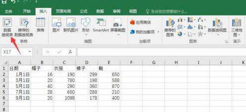
1、进入WPS Office 2016,找到文件所在的位置,打开要处理的文件,进入Excel主界面后,点击插入按钮。

2、点击插入过后,点击最左边数据透视表。
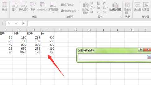
3、进入新界面之后,可以点击一下途中的小图标,缩小该框架。

4、再点击鼠标左键,拖拽你想要设定的区域。这里不仅仅要处理数字,内容也要圈上。
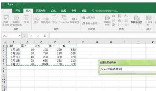
5、圈上之后,在输入框里也会显示出来相应的表格位置。
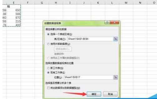
6、再回到刚才的界面,点击最下方确定。
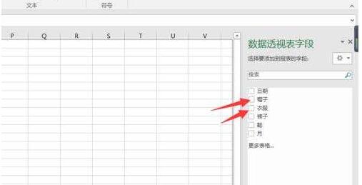
7、这时右侧的数据透视表字段内容,将所有你要计算的内容前面勾上对号。
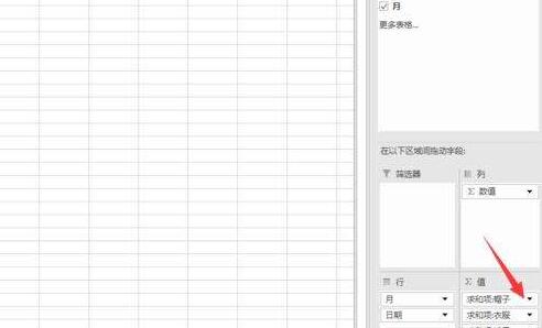
8、如果不是要求和,需要点击下方选项中的倒三角号,再在弹出来的框架中选择值字段设置。
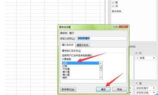
9、选择想要进行的运算模式,求和或者求积或者其他,然后点击确定,回到刚才的界面。
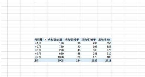
10、最后就可以看到我们设置的数据透视表就完成了,而且直接计算完毕。
注意事项:
1、可以直接利用这个表格。
2、加修改后,也可以把计算结果显示在我们之前表格的下方对应位置。
学完本文WPS Office 2016制作数据透视表的操作流程,是不是觉得以后操作起来会更容易一点呢?